Un-VAE-lievably Simple: Let's Implement Variational Autoencoders
The journey from autoencoders to stable diffusion
Welcome to the series on generative AI. Last week, we learned the intuition behind Variational Auto Encoders (VAEs) and saw some results. This week, we'll cover the math and code so you can build a VAE of your own. Let's get started!
This Week on Gradient Ascent:
What are the odds? Implementing VAEs 🎨
[Consider reading] A Survey on ChatGPT 🧾
[Definitely check out] Overcoming token limits in OpenAI GPT 🛑
[Consider reading] Using LLMs to Research and Plan 🤔
From VAE to Z: A Step-by-Step Guide to Implement your own VAE
Like our forger turned artist Vincent, we learned that VAEs could create original pieces of art by capturing the essence of the great masters while adding their personal expression. In case you missed that, here's a quick recap. VAEs, like traditional autoencoders, have an encoder and a decoder. But, unlike them, VAEs model the underlying distribution of the data. This allows them to create new samples from this distribution. In the following few sections, we'll go through the math and code behind how this is possible and how you, too, can use a VAE to create your own masterpieces.
A Tryst with Randomness
The key ingredient that enables VAEs to generate new samples is the introduction of randomness into the encoding process. The VAE encoder learns to map the input to a distribution instead of a deterministic mapping to achieve this.
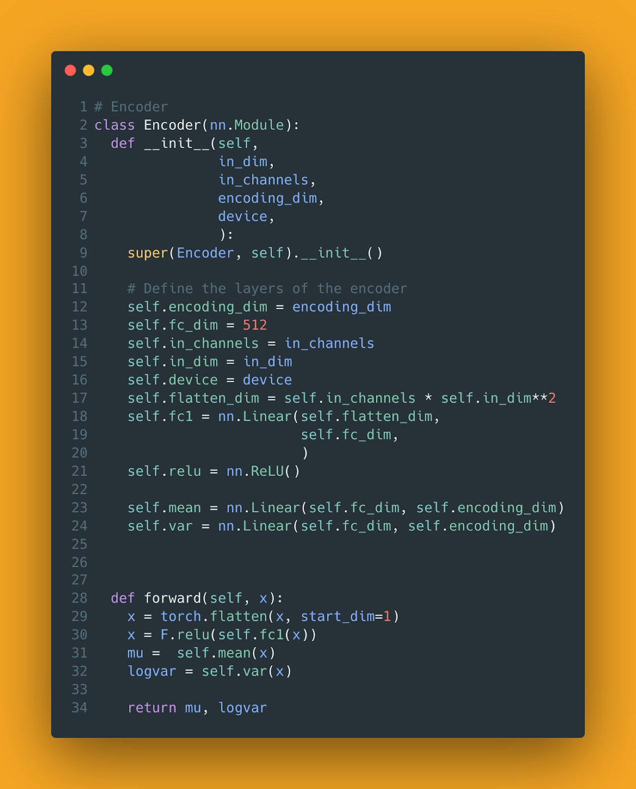
Typically, we use a Gaussian distribution to represent input data in the latent space. So, the encoder learns to estimate the mean and variance of this distribution during the training process. Here's how that looks in code:
Look at lines 31 and 32 above. The encoder learns a mapping to not one but two vectors, one for the mean and one for the standard deviation.
Let the Gradients Flow
Neural networks, like most reasonable humans, learn from feedback. This feedback is provided by comparing their output to the expected result. Essentially, we use the error (the discrepancies between the two) as a signal to update the weights of the network. The error is computed using a loss function. The higher the error, the worse the network's performance. So at every step, the network updates its weights to minimize the error.
But how does it figure out what the new weights should be?
It computes the gradients of the loss function with respect to every weight in the network. Confused? Here's an example that will help you understand better.
Consider a hiker figuring out their way back to base camp after a day in the wilderness. It's gotten dark, and the hiker's headlamp and cell phone have run out of juice. In other words, our hiker friend is blind and in bear country. He needs to get back pronto.
Given that our hiker needs to go downhill as fast as possible, it makes sense to go along the path that has the steepest slope. Unable to see anything, he decides to use his feet as a guide to gauge the steepness of the terrain. Feeling the slope around him with his feet, he figures out which direction to move to descend the valley.
In a neural network, gradients are like the slope of this terrain. They indicate both the direction and magnitude of the steepest increase in the loss function. This is because they are the partial derivatives of the loss function with respect to each of the network's parameters (weights and biases of the network).
To minimize the loss function (the error), we have to move in the opposite direction of the gradients. This is done iteratively by updating the network parameters based on the gradient using an algorithm called gradient descent.
But how do we get the gradients in a neural network?
An algorithm called backpropagation computes this for us. It uses the chain rule from calculus to compute these gradients and works its way back from the output layer to the input layer. Hence the name. Gradient descent then updates the network's weights based on the gradients it receives from backpropagation.
Remember our autoencoder from before? This is how its weights were updated.
But backpropagation requires that the entire network be differentiable. This allows us to compute gradients at each step of the way to update weights. Here's where we hit a problem in the VAE.
Backpropagation works fine for the decoder part of the VAE (which we'll get to next), but then it encounters the sampling section. In the diagram below, you can see it highlighted in orange.
You can't differentiate a sampling process! Uh-oh. So, the backpropagation process stops there! What about the weights of the encoder?
Imagine a set of connected pipes. We want the water to flow from the topmost pipe and reach the faucet at the bottom. But, the sampling process is like a stone stuck in the middle of the pipes, not allowing the water to flow further. What do we do?
Thankfully, researchers devised an ingenious solution to this problem called the "reparameterization" trick.
Instead of directly sampling from the latent distribution, we can first sample from a unit Gaussian distribution (mean = 0, standard deviation = 1). Then, we can shift and scale this by the latent mean and standard deviation as shown below.
The crucial detail here is that reparameterization separates the non-differentiable sampling operation from the rest of the network. Thus, backpropagation can continue without any issues. Again, going back to our water and pipes example, imagine that a plumber pushed the stone so that it moved out of the way. As a result, our water flows freely from top to bottom.
Here's how we can implement reparameterization in Pytorch:
To recap, reparameterization allows VAEs to be trained using gradient descent and learn meaningful latent representations.
Decoding the Masterpieces
The decoder in a VAE is similar to the one found in a regular autoencoder. With the reparameterized sample in hand, the decoder tries to reconstruct the original input. Here's what it looks like in code:
The Full Shabang
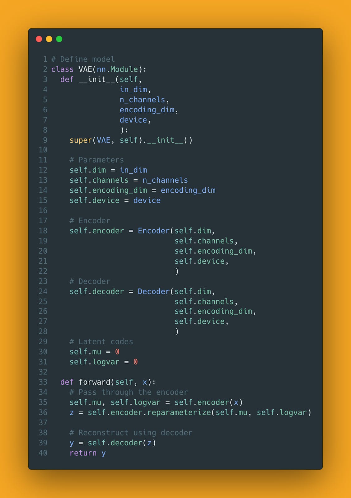
Just so that we're clear on how the VAE looks like, here is the code for the full VAE model:
Pay close attention to the forward function. Notice how we generate z to feed the decoder.
Learning to Balance
To train a VAE, we need a loss function that balances two objectives: reconstructing the input data and regularizing the learned distribution. In simpler terms, the goal is to make sure the VAE learns a smooth and continuous representation of the data, so it can create new, high-quality samples that resemble the original data. Thus, the loss function used to train the model has two components: The reconstruction loss and the KL-divergence.
The reconstruction loss measures the difference between the input and the reconstructed output. We use the mean-squared error in this case, but other options exist.
The KL-divergence acts as a regularization term. It ensures that the distribution the VAE learns stays close to a Gaussian Distribution. This helps in generating diverse samples.
Another way to think about this is as follows. Imagine you're a product manager building a solution for a customer. The customer's expectations are like the standard Gaussian distribution. Your team's design is the learned distribution. Your goal as a product manager is to ensure that the design stays close to the customer's expectations while allowing room for creativity and innovation. That's what the KL-divergence term does in the VAE loss function!
Here's what the loss function looks like in code:
Look at line 5 above. That is the code representation of the KL-divergence:
The derivation is a bit involved, so we'll leave that for another time.
Creating New Artwork
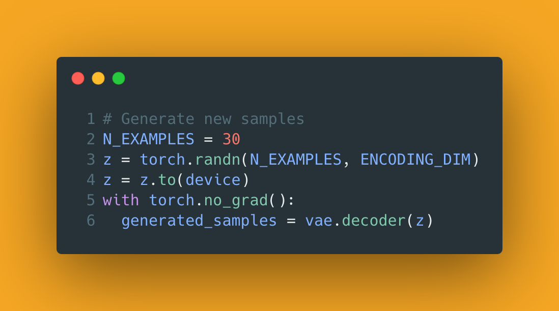
You didn't stick it through this just to learn the workings of a VAE. You want to see it produce new images! So that's what we'll look at next. Once the VAE has been trained, we can use the decoder portion of it to generate new images. All we need to do is generate a random sample from a standard Gaussian distribution and feed that to the decoder. See? easy!
Here's the code to do this:
These are the results the VAE produced:
How cool is that!
In the following article, we'll look at another generative beast.
P.S.: The code for this article can be found here.
Resources To Consider:
A Complete Survey on ChatGPT!
Paper: https://arxiv.org/abs/2304.06488
This excellent survey of ChatGPT covers the underlying technology, applications, and challenges. Given how fast LLM research is moving, this is a great summary to read and understand where things are for now.
Overcoming Token Limits
Token limits are a big blocker for folks building apps using the OpenAI API. In this thread, Kim Woo-yeong walks through some clever strategies to overcome this limit. Build away! Usually, Tweets can be embedded in a substack post. For some reason, they’re refusing to embed. 😉
Link: https://twitter.com/wooing0306/status/1645092115914063872
Experimenting with LLMs to Research, Reflect & Plan
Link: https://eugeneyan.com/writing/llm-experiments/
Eugene Yan shares his experience building a simple assistant using LLMs. His insights are detailed and highly educative. In case you are thinking about building your own smart assistant or are just curious about the process, check out this blog post.


