Vision Transformers: From Idea to Applications Part III
How good are vision transformers at finding objects?
This is part three of a six-part series that Cameron Wolfe and I will write on the Vision transformer and its many applications. I will cover parts 1, 3, and 5, while Cameron will cover parts 2, 4, and 6.
If you just got here and missed the earlier parts, here they are:
Cameron writes an incredible newsletter on deep learning and covers cutting-edge research. Be sure to check out and subscribe to Cameron's newsletter, Deep (learning) focus, here:
Warning: This newsletter edition has a lot of visuals and so may get truncated in email. Consider reading the web version.
This Week on Gradient Ascent:
Where's Waldo, ViT? 🤖
Vision Transformers: Solving the Mystery of Waldo's Whereabouts
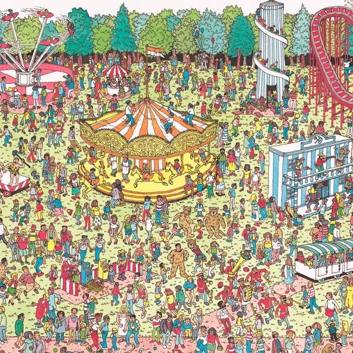
I grew up solving a lot of puzzles - word scrambles, jigsaws, logic. You name it. I loved solving visual puzzles the most; "Where's Waldo?" was my favorite. Nothing gave me more of a rush than finding Waldo in a sea of color. For context, Waldo is a bespectacled guy wearing a red and white striped shirt, a matching winter hat, and a pair of blue jeans. If this sounds easy, I invite you to test your skills on the image below. Can you find Waldo?
Any luck? If you found Waldo, congratulations! You successfully performed object detection. If I'm right, you scanned the image, trying to find every instance of red and white, and then checked to see if you found the other items from Waldo's description.
That's precisely what computers try to do too. Except, they need a lot more help. For starters, I told you that Waldo is a man hidden in a sea of color. Naturally, you thought of a single human figure wearing clothes fitting his description. Unfortunately, a computer doesn't have this context, as all it gets are just streams of pixels. A Waldo to a computer is just the same as a candy cane, a beach towel, or something else that's red and white. Thus, we need to repeatedly show examples of what Waldo looks like and identify where he is in pictures by drawing rectangles around him. These rectangles are meaningfully named bounding boxes.
Detection is a challenging problem
Image classification deals with recognizing "what" an object is. In other words, a classifier doesn't care where the object is. It just cares if it is in the image or not. Object detection, however, deals with "what" an object is and "where" it is in an image. Not just "where" but "where all" it is.
To understand this better, think about an image of zebras1 (or choose your favorite animal from the African savanna). Zebras move in herds, and you'd be hard-pressed to find a single Zebra strutting around the grasslands2. That would only end badly for it.
Let's say you have a detector whose sole purpose of existence is to detect zebras in images. To be good at this gig, it would have to not just detect one zebra but all of them. This opens up a can of worms.
What if a zebra is partially hidden behind a few others? What if there are zebras of different sizes, some in the foreground and some in the distance? Should it return a single box encapsulating all the zebras or one box per zebra? What if it partially detects a zebra and returns an incorrect box? What if it returns duplicate boxes for the same zebra?
These are just some of the many problems that object detectors face. To successfully train a detector, you'll need labeled data that identifies each object's type and provides a tight bounding box to demarcate its position. Here's the kicker.
Deep learning models need a ton of training data, and in the case of object detection, it becomes tough to collect this data. Imagine sitting in a room, drawing rectangles around miscellaneous objects all day, and labeling them. Thankfully, some existing datasets can help us, like MS-COCO.
Waldotron-4000
Let's come back to our Waldo example for a minute. Can you train a model to find Waldo? That's what a creative agency called redpepper did. They trained a robotic arm to spot Waldo. It does surprisingly well.
Here's a rough workflow of what they did. They used OpenCV to find all the faces in the image and then fed that to Google's AutoML solution to discard all the non-Waldo faces. To train this model, they used about 100 hand-labeled examples. That might not seem like much data, but you have to remember that Google's solution already has a strong initialization. It probably leveraged transfer learning to make the Waldo detector rock solid.
I highlighted their workflow to show how many moving parts there are in object detection, even in an almost off-the-shelf version. So, you can imagine how hard it is to build a solution that does this end-to-end.
Object detection has several applications. Surveillance cameras, autofocus in your camera3, medical imaging, counting objects, and self-driving cars, to name just a few. So, it's a problem with a lot of commercial value.
But before we explore how transformers help simplify this task, let's first understand how we can evaluate if a detector is doing its job well.
IOU; Not that way though
A good detector does two things right: It draws a tight bounding box around an object and correctly identifies the type of object. What we need is a metric that can evaluate both of these criteria.
How good are you at drawing rectangles?
IOU, or Intersection Over Union, is a metric that measures how good the detector's predicted bounding boxes are. The idea is straightforward. To evaluate the quality of a predicted box, we compare it with the actual ground truth. In the image below, the green box is the ground truth box, while the red is the predicted box. To calculate the IOU score, we simply calculate the area of intersection between the two boxes and divide it by the area of the union of the two boxes. The higher the IOU, the better the detector predicts bounding boxes. Simply put, a good prediction intersects significantly with the ground truth.
Since the detector is unlikely to get the exact ground truth box, we need to design a way to identify if a predicted box is good and can be used. To do this, we can set an IOU threshold to identify good boxes versus bad ones. For example, if the IOU score for a prediction is greater than 0.5, we'll use that box for further processing.
How good are you at drawing rectangles AND identifying things?
mAP, or mean Average Precision, is the metric commonly used to evaluate object detectors. To understand it, we need to understand a couple of related metrics called precision and recall. These can sound scary, but they're really just common sense measurements.
Precision is the portion of positive predictions that the detector got right. What do I mean by positive here? Let's go back to our detector from earlier, which enjoys detecting zebras. If our detector truly finds a zebra in the image, that is a positive prediction for this detector. Now say we show it an image of a horse and some zebra hanging out. It does its thing and returns bounding boxes for each zebra and the horse. But, it labels the horse as a zebra too. You now have two types of predictions - True positives (calling a zebra a zebra) and false positives (calling a horse a zebra). The precision of our detector is the ratio of true positives to the total number of positives (true and false positives).
In other words, precision measures how accurate the detector's predictions are.
Recall measures how well the detector finds all the positives. Let's say that in our horse and zebra image, there are 6 zebras and just one stallion. Our detector found 5 zebras correctly. But it missed one of them. This missed zebra is called a false negative. The five zebras it detected are true positives. The recall is the ratio of the true positives to all positives (true positives + false negatives).
Our IOU threshold from earlier has a bearing on precision and recall. If we set the IOU threshold higher, we get high-quality boxes. This correlates with higher precision scores. But we'll get fewer detected boxes since we only return the very best. Thus our recall will be lower as there's a chance we miss some true positives because the bounding box associated with that object had a low IOU score. As you can see, it's a tradeoff.
How do we capture how well the model does if the IOU threshold we choose determines the precision and recall values? Simple. We can average the precision over multiple IOU thresholds to get a holistic picture.
That's exactly what mean average precision is! A good detector has a high value of mAP.
Detection before the transformers era
We have enough context now to look at what approaches researchers have tried to build robust object detectors. Since this is a series on transformers, I'll keep this section short. If you'd like to learn the history of object detectors, check out this wonderful paper.
Before transformers, convolutional neural networks (CNNs) were the predominant architecture choice for any vision problem. Object detectors evolved from two-stage detectors to single-stage detectors. Both styles of detectors used CNNs as the backbone architecture.
In two-stage detectors, a set of candidate objects are first proposed, and then the second stage refines these proposals down to the final predictions. Typically, one model extracts these candidate regions, and a second model classifies and refines the bounding boxes for each object. Why not use just the first model, then? Well, the first stage model was fast but inaccurate. It could ensure higher recall but not high precision. The second-stage model was more accurate. It could ensure higher precision. But, it was compute-heavy and slow. Thus, it was used only after candidate proposals were generated by the first model. Some popular two-stage models include RCNN, Fast RCNN, Faster RCNN, and Feature Pyramid Networks (FPN)4.
Single-stage detectors overcame these limitations and consolidated the entire process into one stage (hence the name). These were also fast and lightweight. Popular single-stage detectors include YOLO (I kid you not. It's actually called that), SSD, and RetinaNet.
Transformers, assemble
There are many papers that leverage transformers for object detection, but I want to highlight four5 of them in this article.
Convolution - Transformer hybrid
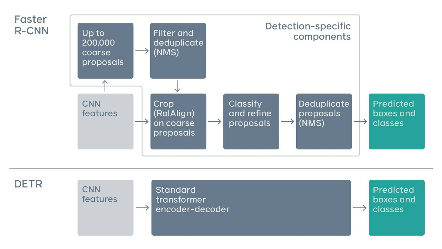
In 2020, MetaAI research released Detection Transformers (DETR). One of the biggest benefits of this model was that inference could be condensed into 50 lines of python code. Prior work typically needed various heuristics to be baked into the mix and thus was clunky. To illustrate this, here's a figure comparing the pipelines of a two-stage Faster R-CNN and DETR. The standard transformer replaced the entire detection-specific stack. Mental right?
Here's what DETR looks like under the hood:
Two interesting tidbits - 1) The ViT paper would not be released for another few months, so this is the first paper that actually integrated transformers in a vision task. 2) This paper used the full transformer (encoder + decoder), unlike subsequent work, which used just the encoder alone.
In DETR, the CNN is used just as a feature extractor, i.e., to find interesting regions in the image. The features extracted from the image are mixed with positional embeddings (recall that, unlike CNNs, transformers don't have positional context for the extracted features).
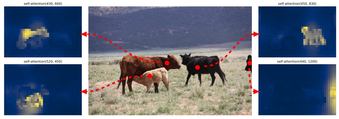
This mixture is passed through a transformer encoder-decoder setup. In addition to the output of the encoder, the decoder also receives object queries (corresponding to the type of objects the image is likely to contain). Self-attention mechanisms enable the transformer to globally reason about the image and specific objects within it. So, it can predict the contents within a bounding box based on other parts of the image. It can also use context from nearby regions in an image to understand relationships between objects. The decoder is connected to fully connected layers that predict an object class and regress its bounding box.
During training, these predictions are compared to ground truth classes and boxes using a bipartite matching algorithm. If that sounds fancy, think of it like the matching exercise we used to do in middle school. You have two columns on a page. Match every item on the left column to the most appropriate item on the right column. In this case, DETR would match every object class and box it predicted to the best candidate from the ground truth.
DETR could predict up to 100 objects but struggled to detect smaller objects in an image. Another paper, titled Deformable DETR, addressed this limitation.
Vision transformer only, please
After the original ViT paper was released, researchers feverishly worked on using the architecture for other vision tasks, such as detection and segmentation. One of the first successful attempts at this produced YOLOS (You Only Look at One Sequence). This work was inspired by DETR but used a ViT-esque architecture for end-to-end detection. Instead of the [CLS] token used by a ViT for classification, YOLOS randomly initialized 100 [DET] tokens to the input image patch embeddings. The authors also used a similar bipartite matching scheme as DETR.
Despite being one of the earliest attempts to use vision transformers for detection, YOLOS performed pretty well when compared to CNNs and DETR. At smaller-sized comparisons, it could beat existing models (at the time).
As the size of the models increased, YOLOS couldn't outperform DETR.
Introducing CNN sensibilities to a ViT
Around the same time that YOLOS was published, researchers from Microsoft introduced the Swin Transformer. This model was inspired by the design of CNNs and combined the power of a transformer with strong priors for visual modeling.
In particular, it introduced three key priors that were previously missing in transformers:
Hierarchy: This helps the transformer recognize objects at different scales. Let's revisit our zebra example. A zebra in the foreground (closer to the camera) will appear larger than one in the distant background. Using a hierarchical structure allows you to capture this. CNN-based methods used a technique called feature pyramids. That's a fancy way of saying, "I have the same image in a bunch of different sizes from small to large, and I'll try to detect the object in each of these images". This gives a model the chance to find an object in at least one of the sizes. The Swin transformer leveraged this technique, but for image patches.
Locality: Unlike language, images are very spatially correlated. Adjacent regions in an image are likely to belong to the same type of object or, at the very least, give us an idea about the relationship between two objects. Swin transformers use shifted windows to compute attention. In particular, the windows within which the Swin transformer computes attention are non-overlapping. They also enable cross-window connections. This makes the Swin transformer consider location priors, but also significantly faster than a traditional ViT (linear vs quadratic complexity, to be exact).
Translational Invariance: You want your detector to find an object, regardless of where in the scene an object might be. This property is called translational invariance. In the Swin transformer design, the researchers add a bias term to the attention formula to make it "translationally semi-invariant," as shown below. It's called semi-invariance because the Swin transformer uses non-overlapping windows and, therefore, cannot be truly translationally invariant.
The Swin transformer was a huge success achieving state-of-the-art results and comfortably beating the previous best model (at the time).
Back to the basics
The final couple of papers I'll share questioned the need for the multistage design that was inherited from CNNs. When we highly customize an architecture, we lose flexibility in exchange for task-specific performance.
Researchers from Google explored whether these customizations were necessary using systematic experiments. The result was a new detection model called UViT (Universal Vision Transformer). They also found that the CNN-based design choices didn't provide strong benefits.
They instead opted to incorporate a simpler design and vary the attention window sizes in the model, as shown below. Their work yielded excellent results while also being reasonably fast.
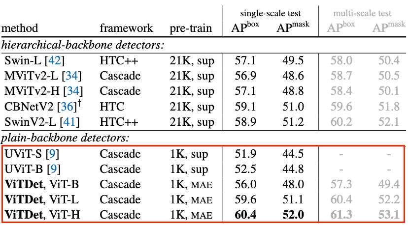
Researchers from MetaAI abandoned hierarchical designs and feature pyramid networks. Instead, they added a simple feature pyramid to the last feature map of the architecture. They also used non-overlapping windows for computing attention and a minimal number of cross-window blocks. The resulting model, called VitDet, achieved amazing results.
While this might seem more complex than UVit, it actually allows for greater flexibility. Why? Transformers are trained in two stages - pre-training and finetuning. The finetuning stage is where we train the model on the desired downstream task. Unlike UViT, which changes the architecture during the pre-training stage, the ViTDet model uses the original ViT architecture as a backbone without explicitly priming it for detection. Thus, the same backbone can be used for a variety of tasks.
Where do we go from here?
Despite the volume of transformer-based research that's been published over the last couple of years, there is still room for improvement in this fascinating architecture. In this regard, text or prompt-based detection models might be an interesting area to explore for future research. Language processing and computer vision are coming closer together, and the transformer has played a vital role in this.
If you stuck it out this far, then you deserve to know where Waldo is in that image way above. Check around the tram in the foreground, and you might find a familiar face there.
I have no idea how I went from red and white stripes to black and white stripes. Mysterious is the mind of man (or just mine).
That happens only in the movie Madagascar.
How else do you think it gets incredible freeze-frame images of that lightning-fast terrier of yours?
We machine learning researchers love our acronyms.
Maybe more ;)


How cool, looking for Waldo (which I gave up on, thank you for revealing his location 😂) then being introduced to object detection was so smart! Another great essay Sairam!
Nice read